The Spacetime Geometry of Diffusion Models

A summary of our work on defining a geometric structure on the latent space of diffusion models using information geometry.

Introduction

Latent generative models - VAEs, GANs, diffusion models - all share a common structure: a latent space and a decoder that maps latent codes to data. In VAEs and GANs, the latent space is typically lower-dimensional than the data, and it has long been understood that equipping it with the right geometry leads to more meaningful distances and more realistic interpolations . But what about diffusion models, where the latent and data spaces share the same dimension?

In this post, we summarize our recent work , where we investigate the geometry of diffusion model latent spaces. We first show an interesting negative result: the standard “pullback” approach, which works well for VAEs, provably collapses in diffusion models, i.e. all shortest paths decode to straight lines. We then introduce a fix: by switching to a stochastic view and treating the (state, time) pair as a point in a latent spacetime, we recover a rich geometric structure using information geometry. The resulting shortest paths, spacetime geodesics, trace minimal sequences of noise-and-denoise edits between data points. We demonstrate two applications: a principled Diffusion Edit Distance between images, and transition path sampling in molecular systems.

A geodesic in spacetime is the shortest path between denoising distributions. As we traverse the curve, the denoising posterior smoothly transitions from one data point to another.

Shortest Paths in Latent Spaces

Before diving into diffusion models, let’s see why geometry matters for latent spaces. Given a latent space \(\mathcal{Z}\) and a decoder \(f: \mathcal{Z} \to \mathcal{X}\), we often want to interpolate between two latent codes \(\mathbf{z}^a\) and \(\mathbf{z}^b\). The simplest approach is linear interpolation - a straight line in \(\mathcal{Z}\). But straight lines in latent space don’t generally map to “realistic” paths in data space. They tend to pass through atypical regions of the distribution, producing unrealistic intermediate samples.A common intuition is that straight-line interpolations fail because they cut through *low*-density regions. The reality is more subtle. For instance, with a Gaussian prior, straight lines pass through the *center* — a high-density region. But high density does not mean typical: in high dimensions, the mode of a distribution can be far from where samples actually concentrate. We explore this phenomenon in detail in a companion blog post , where we show that the highest-density regions of diffusion models correspond to blurry, cartoon-like images rather than realistic data.

The solution is to define a notion of infinitesimal distance in \(\mathcal{Z}\) that captures the structure of the data. Given a way to measure the “cost” \(d(\mathbf{z}, \mathbf{z} + d\mathbf{z})\) of an infinitesimal step, the “shortest path” is no longer a straight line, but a geodesic - a curve that minimizes the total cost of traversal. Different choices of infinitesimal distance lead to different geodesics, and hence different notions of what it means to interpolate between two latent codes.

Different choices of infinitesimal distance lead to different geodesics between the same endpoints.

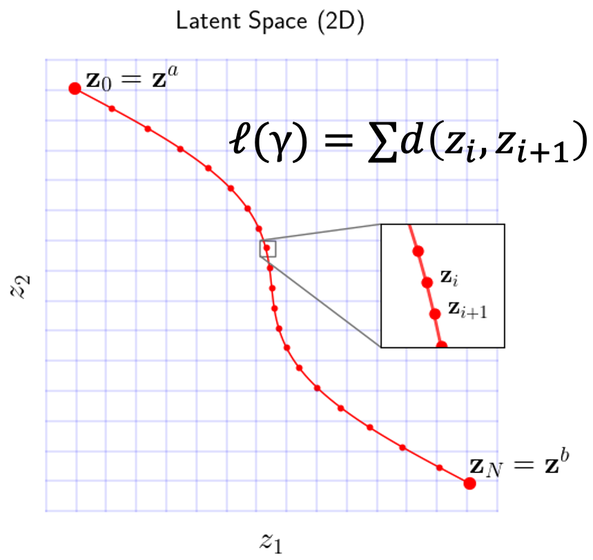
For a discretized curve \(\gamma = (\mathbf{z}_0, \ldots, \mathbf{z}_N)\), finding the geodesic amounts to minimizing the energy

\[\mathcal{E}(\gamma) \approx \frac{N}{2} \sum_{i=0}^{N-1} d^2(\mathbf{z}_i, \mathbf{z}_{i+1}),\]

where \(d\) is the local infinitesimal distance. The key question is: how should we define \(d\)?

Pullback Geometry

A natural choice, well-studied in the context of VAEs , is the pullback metric. Suppose we have a deterministic decoder \(f: \mathcal{Z} \to \mathcal{X}\). The pullback metric defines the infinitesimal distance between nearby latent codes as the Euclidean distance between their decoded outputs:

\[d(\mathbf{z}, \mathbf{z} + d\mathbf{z}) = \|f(\mathbf{z}) - f(\mathbf{z} + d\mathbf{z})\|.\]

With this choice, geodesics try to keep the decoded curve as smooth as possible - they follow the “surface” of the data manifold rather than cutting through empty space. This works beautifully for VAEs, where the latent space is lower-dimensional than the data space, producing more realistic interpolations than linear baselines.

Diffusion Models Recap

Recall that diffusion models gradually transform a data distribution \(q\) into noise via a forward process

\[p(\mathbf{x}_t \mid \mathbf{x}_0) = \mathcal{N}(\mathbf{x}_t \mid \alpha_t \mathbf{x}_0, \sigma_t^2 I),\]

where \(\alpha_t, \sigma_t\) control how quickly information is destroyed. At the final time \(T\), we reach approximately pure noise: \(p_T \approx \mathcal{N}(0, \sigma_T^2 I)\).

To generate data, we reverse this process. There are two flavors:

• Deterministic (PF-ODE): \(d\mathbf{x} = \left(f_t \mathbf{x} - \tfrac{1}{2}g_t^2 \nabla \log p_t(\mathbf{x})\right) dt\), which defines a bijection \(\mathbf{x}_T \mapsto \mathbf{x}_0(\mathbf{x}_T)\).
• Stochastic (Reverse SDE): \(d\mathbf{x} = \left(f_t \mathbf{x} - g_t^2 \nabla \log p_t(\mathbf{x})\right) dt + g_t d\overline{W}_t\), which defines a denoising posterior distribution \(p(\mathbf{x}_0 \mid \mathbf{x}_t)\) for each noisy input — the distribution over clean data consistent with the noisy observation.

Both require the score function \(\nabla \log p_t(\mathbf{x})\), which is approximated by a neural network. The deterministic decoder gives us a single clean image for each noise vector; the stochastic decoder gives an entire denoising posterior over possible clean images.

Pullback Geometry Fails for Diffusion Models

Armed with the pullback metric and a deterministic PF-ODE decoder \(\mathbf{x}_T \mapsto \mathbf{x}_0(\mathbf{x}_T)\), one might hope to get nice curved geodesics between images, as in VAEs. Unfortunately, this does not work.

Theorem. Pullback geodesics in diffusion models decode to straight lines in data space.

Why? The pullback energy of a latent curve \(\gamma\) only depends on the decoded curve (see the proof in ):

\[\mathcal{E}_{\text{PB}}(\gamma) = \frac{1}{2}\int_0^1 \left\| \frac{d}{ds}\mathbf{x}_0(\gamma_s) \right\|^2 ds.\]

The minimizer is always the constant-speed straight line \(\mathbf{x}_s = (1-s)\mathbf{x}^a + s\mathbf{x}^b\) in data space. Since the PF-ODE is a bijection, this line has a unique latent preimage, which is therefore the pullback geodesic. The result: pullback geodesics may curve in noise space, but they always decode to straight lines in data space, completely ignoring the structure of the data manifold.

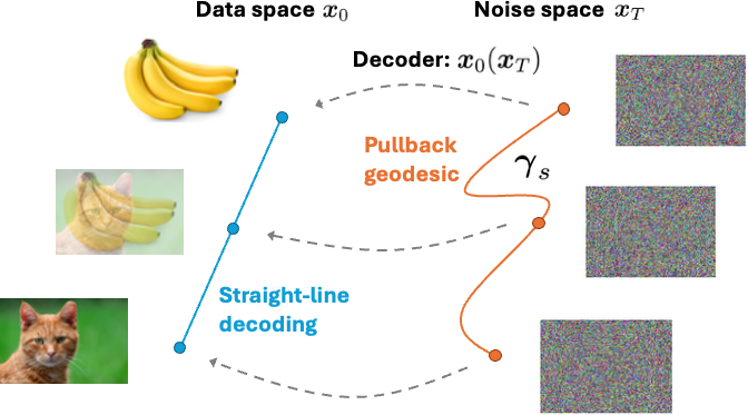
The pullback geodesic may curve in the latent (noise) space, but its decoding is always a straight line in data space.

The root cause is that, unlike VAEs, diffusion models have latent and data spaces of equal dimension. The decoder operates directly in the ambient space, and without a dimensionality bottleneck, it cannot capture intrinsic data structure through pullback alone.

Take-home: The standard pullback metric is fundamentally unsuitable for diffusion models. We need a different approach.

The Spacetime Alternative

What is the Latent Space of a Diffusion Model?

In diffusion models, there are many possible choices for the “latent” representation: we could use \(\mathbf{x}_t\) at any noise level \(t\). But fixing a single \(t\) is arbitrary, and at \(t = T\) the representation is essentially meaningless, i.e. the forward process is memoryless, so \(p(\mathbf{x}_0 \mid \mathbf{x}_T) \approx q(\mathbf{x}_0)\), independent of \(\mathbf{x}_T\).

Instead, we propose to consider all noise levels simultaneously. A point in our latent space is a spacetime coordinate

\[\mathbf{z} = (\mathbf{x}_t, t) \in \mathbb{R}^D \times (0, T],\]

pairing a noisy sample with its noise level. For \(D\)-dimensional data, this yields a \((D+1)\)-dimensional spacetime. Clean data \(\mathbf{x}\) lives at \((\mathbf{x}, 0)\), the boundary of the spacetime.

What is the Decoder?

In the spacetime view, each latent point \(\mathbf{z} = (\mathbf{x}_t, t)\) indexes a denoising distribution \(p(\mathbf{x}_0 \mid \mathbf{x}_t)\), which is the distribution over clean data that could have produced the noisy observation \(\mathbf{x}_t\) at noise level \(t\). The “decoder” is no longer a single point, but an entire probability distribution. This is key: instead of comparing decoded points, we compare decoded distributions.

Information Geometry

The goal is the same as with the pullback: we want to measure how much the “decoding” changes when we take an infinitesimal step in the latent space. The difference is that the decoder now outputs a distribution rather than a point, so we need to replace the Euclidean distance with a measure of discrepancy between distributions. The natural choice from information geometry is the KL divergence:

\[d^2(\mathbf{z}, \mathbf{z} + d\mathbf{z}) = \text{KL}\left[p(\mathbf{x}_0 \mid \mathbf{z}) \| p(\mathbf{x}_0 \mid \mathbf{z} + d\mathbf{z})\right].\]

This is the Fisher-Rao metric.More precisely, the KL divergence to second order is $$\text{KL}[p(\mathbf{x}_0 \mid \mathbf{z}) \| p(\mathbf{x}_0 \mid \mathbf{z} + d\mathbf{z})] = \frac{1}{2} d\mathbf{z}^\top G_{\text{IG}}(\mathbf{z}) \, d\mathbf{z} + o(\|d\mathbf{z}\|^2)$$, where $$G_{\text{IG}}(\mathbf{z}) = \mathbb{E}_{\mathbf{x}_0 \sim p(\mathbf{x}_0 \mid \mathbf{z})} \left[ \nabla_{\mathbf{z}} \log p(\mathbf{x}_0 \mid \mathbf{z}) \, \nabla_{\mathbf{z}} \log p(\mathbf{x}_0 \mid \mathbf{z})^\top \right]$$ is the Fisher information matrix. To summarize, both the pullback and the Fisher-Rao metric aim to measure the same thing — how much the decoding changes — but they formulate it differently depending on the nature of the decoder:

	Deterministic Decoder	Stochastic Decoder
Decoder output	A point \(f(\mathbf{z})\)	A distribution \(p(\mathbf{x}_0 \mid \mathbf{z})\)
Infinitesimal discrepancy	\(||f(\mathbf{z}) - f(\mathbf{z}+d\mathbf{z})||^2\)	\(\text{KL}[p(\cdot \mid \mathbf{z}) || p(\cdot \mid \mathbf{z}+d\mathbf{z})]\)
Metric name	Pullback	Fisher-Rao

A geodesic under the Fisher-Rao metric is the path that minimizes the total change in denoising posterior — exactly what we want.

Computing Geodesics in Practice

Usually, computing geodesics under the Fisher-Rao metric is only tractable for simple parametric families (e.g., Gaussians). The denoising distributions in diffusion models are complex, high-dimensional, and non-Gaussian. So how can we make this work?

The key insight is that the denoising distributions form an exponential family. Despite being complicated, \(p(\mathbf{x}_0 \mid \mathbf{x}_t)\) can always be written asThis follows from Bayes' rule and the Gaussian form of the forward kernel. The data distribution \( q(\mathbf{x}_0) \) plays the role of the base measure, and the Gaussian forward kernel contributes the exponential interaction term.

\[p(\mathbf{x}_0 \mid \mathbf{z}) = q(\mathbf{x}_0) \exp\left(\boldsymbol{\eta}(\mathbf{z})^\top T(\mathbf{x}_0) - \psi(\mathbf{z})\right),\]

with natural parameter \(\boldsymbol{\eta}(\mathbf{x}_t, t) = \left(\frac{\alpha_t}{\sigma_t^2}\mathbf{x}_t, -\frac{\alpha_t^2}{2\sigma_t^2}\right)\) and sufficient statistic \(T(\mathbf{x}_0) = (\mathbf{x}_0, \|\mathbf{x}_0\|^2)\). This is the same exponential structure as a Gaussian, but with the data distribution \(q\) as the base measure instead of a flat Lebesgue measure.

Why does this matter? Because for exponential families, the curve energy simplifies dramatically. The energy of a discretized curve \(\gamma = (\mathbf{z}_0, \ldots, \mathbf{z}_{N-1})\) is

\[\mathcal{E}(\gamma) \approx \frac{N-1}{2} \sum_{n=0}^{N-2} \left(\boldsymbol{\eta}(\mathbf{z}_{n+1}) - \boldsymbol{\eta}(\mathbf{z}_n)\right)^\top \left(\boldsymbol{\mu}(\mathbf{z}_{n+1}) - \boldsymbol{\mu}(\mathbf{z}_n)\right),\]

where \(\boldsymbol{\mu}(\mathbf{z}) = \mathbb{E}[T(\mathbf{x}_0) \mid \mathbf{z}] = \left(\mathbb{E}[\mathbf{x}_0 \mid \mathbf{z}], \, \mathbb{E}[\|\mathbf{x}_0\|^2 \mid \mathbf{z}]\right)\) is the expectation parameter. The natural parameter \(\boldsymbol{\eta}\) is known in closed form, and the expectation parameter \(\boldsymbol{\mu}\) can be estimated from the denoiser network \(\hat{\mathbf{x}}_0(\mathbf{x}_t)\) using Tweedie’s formula and a single Jacobian-vector product.

This means spacetime geodesics are simulation-free: we never need to run the reverse SDE. For a curve discretized into \(N\) points, we only need \(N\) forward passes through the denoiser. In practice, we parameterize \(\gamma\) as a cubic spline with fixed endpoints and minimize \(\mathcal{E}(\gamma)\) via gradient descent.

Take-home: Denoising distributions form an exponential family, which makes the Fisher-Rao energy tractable. Geodesics can be computed efficiently with just forward passes of the denoiser.

Application: Diffusion Edit Distance

The spacetime geometry induces a principled distance between data points. We identify a clean datum \(\mathbf{x}\) with the spacetime point \((\mathbf{x}, 0)\), corresponding to the Dirac denoising distribution \(\delta_{\mathbf{x}}\). Given two data points \(\mathbf{x}^a\) and \(\mathbf{x}^b\), the Diffusion Edit Distance (DiffED) is defined as

\[\text{DiffED}(\mathbf{x}^a, \mathbf{x}^b) = \ell(\gamma),\]

where \(\gamma\) is the spacetime geodesic connecting \((\mathbf{x}^a, 0)\) and \((\mathbf{x}^b, 0)\).In practice, we anchor the endpoints at a small \(t_{\min} > 0 \) rather than exactly at 0, because at \( t = 0 \) the denoising distributions collapse to Dirac deltas, making the Fisher-Rao distance infinite.

The interpretation is intuitive: a spacetime geodesic links two clean data points through intermediate noisy states. It traces the minimal sequence of edits: add just enough noise to forget information specific to \(\mathbf{x}^a\), then denoise to introduce information specific to \(\mathbf{x}^b\). The path length quantifies the total “edit cost”, measured by how much the denoising distribution changes along the way. As endpoint similarity decreases, the geodesic passes through noisier intermediate states—the model needs to “forget” more before it can “reconstruct” the target.

Spacetime geodesics between images. Each row shows a geodesic between two clean images. The path passes through noisy intermediate states: more noise is needed when the endpoints are more dissimilar.

We evaluated DiffED on ImageNet images using the pretrained EDM2 model . Interestingly, DiffED has only weak correlation (-7%) with the perceptual similarity metric LPIPS , but correlates at 53% with the structural similarity index SSIM . This suggests that DiffED captures a notion of “structural edit cost” that is distinct from perceptual similarity - it measures how much the generative model needs to change its beliefs, rather than how similar the images look to a human.

Take-home: DiffED measures the minimal “noise-and-denoise” editing cost between two data points, as determined by the diffusion model’s own learned structure.

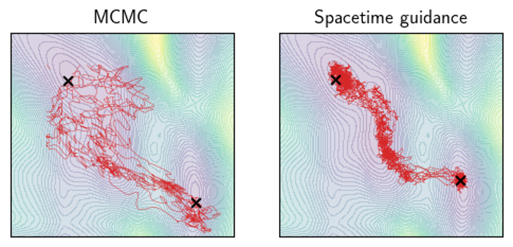
Application: Transition Path Sampling

Beyond images, the spacetime framework has a natural application in molecular dynamics: transition path sampling. Given a molecular system described by a Boltzmann distribution \(q(\mathbf{x}) \propto \exp(-U(\mathbf{x}))\), the goal is to find plausible transition paths between two low-energy states (e.g., two stable configurations of a molecule), navigating around the high-energy barriers that separate them.

Here’s the key connection. When the data distribution is Boltzmann, the denoising distribution is also Boltzmann:

\[p(\mathbf{x}_0 \mid \mathbf{x}_t) \propto \exp\left(-U(\mathbf{x}_0 \mid \mathbf{x}_t)\right), \qquad U(\mathbf{x}_0 \mid \mathbf{x}_t) = U(\mathbf{x}_0) + \tfrac{1}{2}\text{SNR}(t)\|\mathbf{x}_0 - \mathbf{x}_t/\alpha_t\|^2,\]

where \(\text{SNR}(t) = \alpha_t^2 / \sigma_t^2\). This conditional energy combines the true potential with an additional bias toward \(\mathbf{x}_t / \alpha_t\) - at low noise (high SNR), the distribution is concentrated near the latent; at high noise (low SNR), it approaches the unconditional Boltzmann.

Our method proceeds in two steps:

1. Compute a spacetime geodesic between the two low-energy states \(\mathbf{x}^1_0\) and \(\mathbf{x}^2_0\). This provides an optimal interpolation of denoising distributions from \(\delta_{\mathbf{x}^1_0}\) to \(\delta_{\mathbf{x}^2_0}\).
2. Sample transition paths by running annealed Langevin dynamics along the geodesic. Starting from \(\mathbf{x} = \mathbf{x}^1_0\), we iterate over the spacetime curve points \(\gamma_n\), taking a few Langevin steps targeting \(p(\mathbf{x} \mid \gamma_n)\) at each point. Since consecutive distributions along the geodesic change smoothly (that is what geodesics are optimized for!), the current sample is always a good initialization for the next Langevin chain.

How denoising posteriors change along the spacetime geodesic in the transition path sampling example. Right: a point traversing the spacetime geodesic. Left: the corresponding denoising posterior at each point along the curve. The geodesic provides a smooth interpolation of distributions between the two low-energy states.

We tested this on Alanine Dipeptide, a standard benchmark in the transition path sampling literature . Our method achieves a MaxEnergy of \(37.36 \pm 0.60\), very close to the numerical lower bound of \(36.42\), and significantly better than MCMC baselines (\(42.54 \pm 7.42\)) and Doob’s Lagrangian (\(66.24 \pm 1.01\)). Crucially, it requires orders of magnitude fewer energy evaluations (16M vs. 1.29B for the best MCMC variant).

Transition paths generated using the spacetime geodesic framework. The paths successfully navigate around high-energy barriers between two stable molecular configurations.

Method	MaxEnergy (↓)	# Evaluations (↓)
Lower Bound	36.42	N/A
MCMC-fixed-length	42.54 ± 7.42	1.29B
MCMC-variable-length	58.11 ± 18.51	21.02M
Doob’s Lagrangian	66.24 ± 1.01	38.4M
Spacetime geodesic (Ours)	37.36 ± 0.60	16M (+16M)

Qualitative comparison of transition paths generated by our method and baselines.

Constrained Transitions

A powerful feature of our framework is the ability to incorporate constraints on the transition paths. By adding a penalty term to the energy minimization

\[\min_\gamma \left[ \mathcal{E}(\gamma) + \lambda \int_0^1 h(\gamma_s) \, ds \right],\]

we can enforce additional properties:

• Low-variance transitions: Penalizing low SNR along the path forces the geodesic to stay at higher SNR, which concentrates the denoising posterior and yields more repeatable trajectories.
• Region avoidance: By encoding a “forbidden zone” as a denoising distribution \(p(\cdot \mid \mathbf{z}^*)\) and penalizing proximity to it (via KL divergence), we can steer transition paths away from undesirable regions of the data space.

Both variants are demonstrated in , showing that the spacetime framework flexibly accommodates domain-specific constraints.

Take-home: Spacetime geodesics provide a principled guide for transition path sampling, and the framework naturally extends to constrained variants.

Conclusion

We presented a geometric perspective on the latent space of diffusion models. The standard pullback approach provably collapses, always producing straight-line interpolations in data space. By switching to a stochastic view and introducing the latent spacetime \((\mathbf{x}_t, t)\) equipped with the Fisher-Rao metric, we recover a rich and tractable geometric structure. The key theoretical insight, that denoising distributions form an exponential family, makes geodesic computation practical even for high-dimensional image models.

The resulting framework yields two concrete applications: a Diffusion Edit Distance that measures the minimal noise-and-denoise editing cost between data points, and a transition path sampling method that outperforms specialized baselines in molecular simulations. We believe this geometric perspective opens up further directions, including improved sampling strategies and extensions to discrete or Riemannian diffusion models.