Understanding Likelihood in Diffusion Models
A summary of our two recent articles on estimating and controlling likelihood in diffusion models.
Introduction
In this post, we dive into insights from our two recent works on diffusion models. In the first one
Diffusion Models Recap
A key mechanism in diffusion models
\begin{equation} d\mathbf{x}_t = f(t)\mathbf{x}_t dt + g(t)d W_t \qquad \mathbf{x}_0 \sim p_0, \end{equation}
where \(f, g\) are scalar functions and \(W\) is the Wiener process. Remarkably, this process is reversible! The reverse SDE
\begin{equation}\label{eq:rev-sde} d\mathbf{x}_t = (f(t)\mathbf{x}_t - g^2(t)\nabla \log p_t(\mathbf{x}_t)) dt + g(t)d \overline{W}_t \qquad \mathbf{x}_T \sim p_T, \end{equation}
where \(\overline{W}\) is the Wiener process going backwards in time and \(\nabla \log p_t(\mathbf{x}_t)\) is the score function, which can be accurately approximated with a neural network
Rather surprisingly, it turns out that there exists an equivalent deterministic process
\begin{equation}\label{eq:pf-ode} d\mathbf{x}_t = (f(t)\mathbf{x}_t - \frac{1}{2}g^2(t)\nabla \log p_t(\mathbf{x}_t)) dt \qquad \mathbf{x}_T \sim p_T, \end{equation}
which is also guaranteed to generate a sample \(\mathbf{x}_0 \sim p_0\).
Score matching
Diffusion models are typically trained using a score matching objective, which seeks to approximate the score function \(\nabla \log p_t(\mathbf{x})\) using a neural network \(\mathbf{s}_\theta(\mathbf{x}, t)\):
\[\begin{equation}\label{eq:sm-obj} \mathbb{E}_{t, \mathbf{x}_0, \mathbf{x}_t} \Big[ \lambda(t) \|\mathbf{s}_\theta(\mathbf{x}_t, t) - \nabla \log p_t(\mathbf{x}_t)\|^2 \Big], \end{equation}\]where \(\lambda(t)\) is a weighting function. Interestingly, with an appropriate choice of \(\lambda(t)=g^2(t)\), score matching corresponds to maximum likelihood training
What is Log-Density?
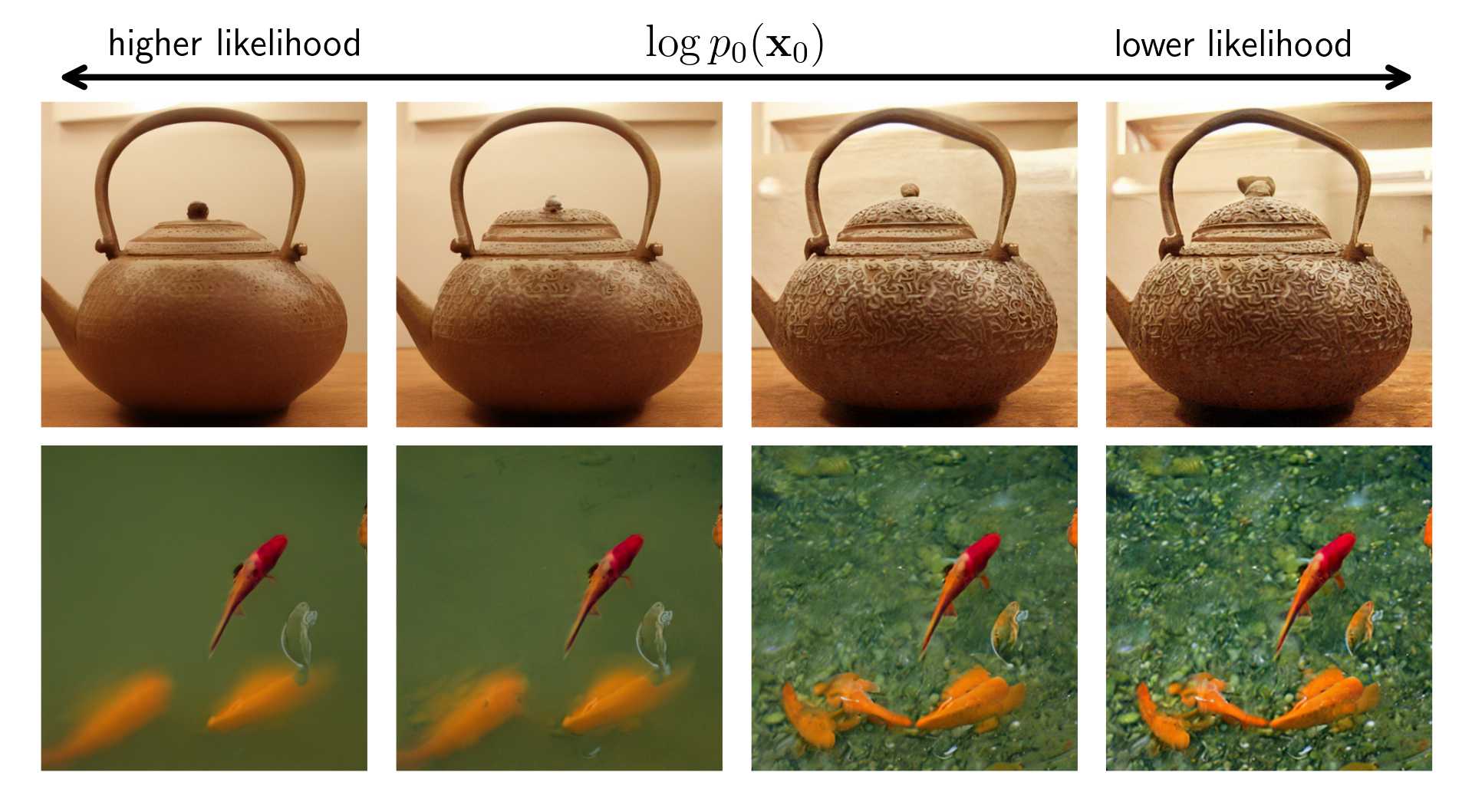
Since diffusion models are likelihood-based models, they aim to assign high likelihood to training data and, by extension, low likelihood to out-of-distribution (OOD) data. Intuitively, one might think that log-density is a reliable measure of whether a sample lies in or out of the data distribution.
However, prior research
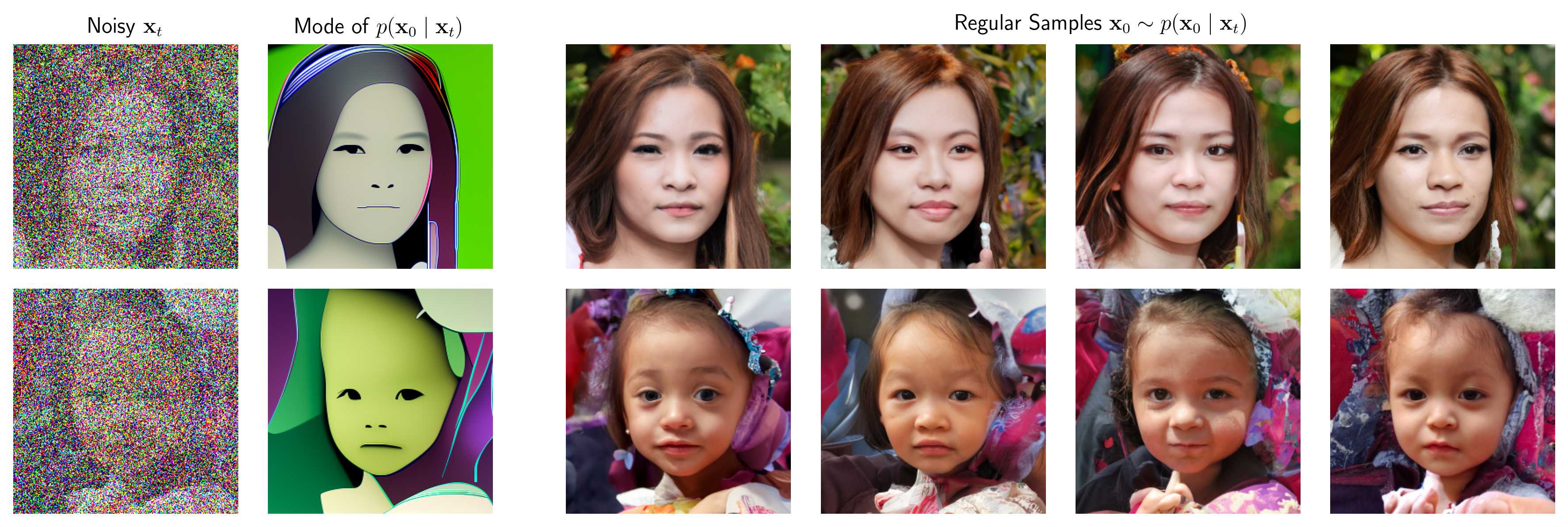
We derive a theoretical mode-tracking ODE and its efficient approximation - the high-density (HD) sampler, which allows us to explore the regions of high density. Specifically, it is an ODE, which converges to the approximate mode of \(p_t(\mathbf{x}_0 \mid \mathbf{x}_t)\) for any starting point \(\mathbf{x}_t\).
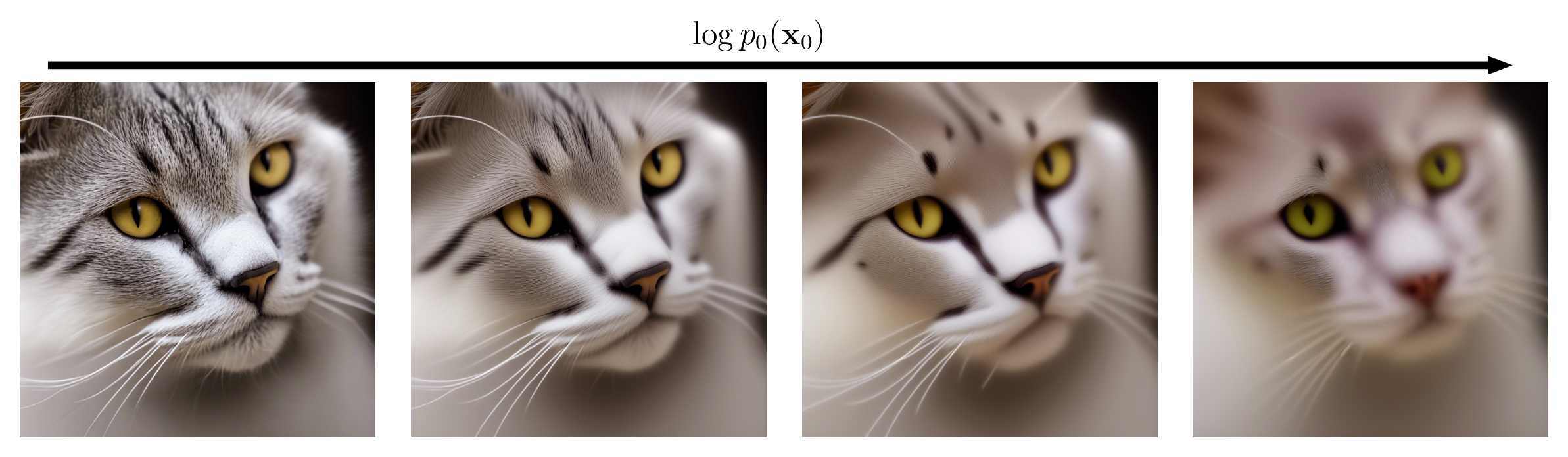
We use the HD-sampler on image diffusion models to investigate the highest-likelihood regions. Surprisingly, these are occupied by cartoon-like drawings or blurry images—patterns that are absent from the training data. Additionally, we observe a strong correlation between negative log-density and PNG image size, revealing that, for image data, negative log-likelihood essentially measures information content or detail, rather than “in-distribution-ness”.
Why Does This Happen?
While we don’t have a full understanding of why the blurry and cartoon-like images occupy the highest-density regions, we discuss several factors that might contribute to this phenomenon.
Model’s Loss Function and Out-of-Distribution Freedom
Diffusion models are trained with variants of the score-matching objective \eqref{eq:sm-obj}, meaning that their loss is optimized only for in-distribution images. However, the model defines the density everywhere, including points outside the distribution which are never seen during training. This gives the model freedom in how it assigns the likelihood to atypical samples such as blurry or cartoon-like ones.
Information Theory and Compressibility
Information theory suggests that high-likelihood images should be more compressible, which translates to low-detail in the context of images. While the exact role of information theory in this context remains unclear, it aligns well with what we observe: the highest-likelihood images are low-detail, simple, and lacking in complex textures, which makes them look like cartoons or appear blurry.
The Density Trade-Off
The set of realistic images is vast. Some are high-detail, while others are low-detail, but the total number of high-detail images is significantly greater due to their higher number of degrees of freedom. Since probability density must integrate to 1, this forces the model to assign lower likelihood to high-detail images simply because there are so many of them. Consider images of: apple on a plain background versus a tree with countless variations of leaves and grass: both are realistic, but the latter has vastly more possible instances, necessitating a lower individual density per image.
The Branching Tree Hypothesis
Recent work
High-Dimensional Distributions and Mode “Paradoxes”
Finally, it is important to recognize that the fact that the highest-density points look very different from regular samples is not unusual in high-dimensional probability distributions. A classic example is the standard \(D\)-dimensional Gaussian: its mode is at the origin, but as dimensionality increases, almost all samples are concentrated on a thin spherical shell at radius \(\sqrt{D}\). Sampling close to the mode (zero vector) has an exponentially vanishing probability as \(D\) grows
Now that we have a better understanding of what density means in diffusion models, we will now discuss how it is actually estimated in practice.
How to Estimate Log-Density?
Estimating the log-density of a generated sample \(\mathbf{x}_0\) boils down to tracking how the marginal log-densities changed over the sampling trajectory:
\[\log p_0(\mathbf{x}_0) = \log p_T (\mathbf{x}_T) - \left( \log p_T(\mathbf{x}_T) - \log p_0(\mathbf{x_0}) \right) = \underbrace{\log p_T(\mathbf{x}_T)}_{\text{known analytically}} + \int_T^0 \underbrace{d\log p_t(\mathbf{x}_t)}_{\text{log-density change}}\]and the log-density change \(d \log p_t(\mathbf{x}_t)\) depends on how we sample. Sampling in diffusion models can be categorized along two main axes:
1. Deterministic vs Stochastic Sampling
Diffusion models generate samples by reversing the forward noising process in two ways:
- Deterministic sampling: Uses smooth, noise-free trajectories of PF-ODE \eqref{eq:pf-ode}.
- Stochastic sampling: Uses noisy trajectories of Reverse SDE \eqref{eq:rev-sde}.
While deterministic sampling is often preferred for efficiency, stochastic sampling can enhance diversity by producing multiple possible reconstructions of the same noisy input.
2. Original vs Modified Dynamics
Sampling with PF-ODE or the Reverse SDE ensures that each intermediate sample \(\mathbf{x}_t\) correctly follows the correct distribution \(p_t\) at every time step. We call this sampling with “original dynamics”.
However, sticking to the original dynamics does not allow us to influence the likelihood of generated samples at \(t=0\). As we will see, extending log-density estimation to modified dynamics, where we alter the drift or diffusion terms of the sampling process, enables precise control over \(\log p_0(\mathbf{x}_0)\). This is crucial for manipulating image characteristics such as detail and sharpness.
We define:
- Original Dynamics: The sampling process follows either the PF-ODE or Reverse SDE exactly, using the learned score function without modification.
- Modified Dynamics: The sampling process deviates from these standard dynamics by altering the drift or diffusion terms.
Previously, \(d \log p_t(\mathbf{x}_t)\) was only known for deterministic sampling under original dynamics—i.e., along PF-ODE trajectories
In
- Stochastic Sampling with Original Dynamics: We derive how log-density evolves along stochastic Reverse SDE trajectories.
Interestingly, we prove that, in contrast to the deterministic case, replacing the true score function \( \nabla \log p_t(\mathbf{x}) \) with an estimate \( \mathbf{s}_\theta (\mathbf{x}, t) \) makes the log-density estimation biased. This bias is given by the estimation error of the score function. - Deterministic Sampling with Modified Dynamics: We show how log-density can be estimated not just for PF-ODE trajectories but for any deterministic trajectory.
Finally, in
- Stochastic Sampling with Modified Dynamics: We prove that \(d \log p_t(\mathbf{x}_t)\) can be estimated for any stochastic trajectory, not just those following the Reverse SDE. This establishes a completely general framework for log-density estimation under any sampling procedure.
The following table summarizes these advancements:
| Sampling Mode | Original Dynamics (PF-ODE / Reverse SDE) | Any Dynamics (Modified ODE / SDE) |
|---|---|---|
| Deterministic | Prior work | Ours |
| Stochastic | Ours | Ours |
Since stochastic trajectories generalize deterministic ones, our final result in
Note that
- For \(\mathbf{u}_t(\mathbf{x})=f(t)\mathbf{x} - g^2(t)\nabla \log p_t(\mathbf{x}),\: G_t(\mathbf{x}) = g(t)I\), we get the Reverse SDE \eqref{eq:rev-sde},
- For \(\mathbf{u}_t(\mathbf{x})=f(t)\mathbf{x} - \frac{1}{2}g^2(t)\nabla \log p_t(\mathbf{x}),\:G_t(\mathbf{x})=\mathbf{0}\), we get the PF-ODE \eqref{eq:pf-ode},
- For \(\mathbf{u}_t(\mathbf{x})=f(t)\mathbf{x} - \frac{1}{2}g^2(t) \eta \nabla \log p_t(\mathbf{x}),\:G_t(\mathbf{x})=\mathbf{0}\), we get a new ODE, which is biased towards higher or lower values of log-density, depending on the value of \(\eta\).
In the next section, we show how this ability to estimate log-density under any dynamics enables us to actively control it, allowing for precise manipulation of image detail in diffusion models.
How to Control Log-Density?
The simplest approach to controlling log-density is to manipulate the latent code. Note that the PF-ODE defines the solution map \(\mathbf{x}_T \mapsto \mathbf{x}_0(\mathbf{x_T})\). One can thus define the objective as a function of the latent code:
\[\mathcal{J}(\mathbf{x}_T) = \log p_0 (\mathbf{x}_0(\mathbf{x}_T)),\]which can be directly optimized by differentiating through the ODE solver
We will discuss how precise density control can be achieved without extra cost by modifying the sampling dynamics, both deterministic and stochastic.
Density Guidance: A Principled Approach to Controlling Log-Density
In
which defines the marginal distributions \(p_t\). We want to find a modified sampling ODE \(d\mathbf{x}_t=\tilde{\mathbf{u}}_t(\mathbf{x}_t)dt\) to enforce
\[\begin{equation}\label{eq:logp-b} d \log p_t(\mathbf{x}_t) = b_t(\mathbf{x}_t)dt \end{equation}\]for a user-defined function \(b_t\). We show that the solution that satisfies this and diverges from the original drift the least is given by
\[\begin{equation} \tilde{\mathbf{u}}_t(\mathbf{x})=\mathbf{u}_t(\mathbf{x}) + \underbrace{\frac{\operatorname{div}\mathbf{u}_t(\mathbf{x}) + b_t(\mathbf{x})}{\|\nabla \log p_t(\mathbf{x})\|^2}\nabla \log p_t(\mathbf{x})}_{\text{log-density correction}}. \end{equation}\]Note that when \(b_t(\mathbf{x}) = -\operatorname{div}\mathbf{u}_t(\mathbf{x})\), we recover the original dynamics \(\tilde{\mathbf{u}}_t = \mathbf{u}_t\). For \(b_t(\mathbf{x}) < -\operatorname{div}\mathbf{u}_t(\mathbf{x})\), we get a model biased towards higher values of likelihood. In practice, this formula is most relevant to diffusion models because we already have (an approximation of) \(\nabla \log p_t(\mathbf{x})\). This is why in the following sections we assume the diffusion model with \(\mathbf{u}_t\) given by \eqref{eq:pf-ode}. The same framework can be used for any continuous-time flow model, provided that the score function is known.
How to choose \(b_t\)?
While density guidance theoretically allows arbitrary changes to log-density, practical constraints must be considered. Log-density changes that are too large or too small can lead to samples falling outside the typical regions of the data distribution. We show that a carefully chosen \(b_t\) allows control of the log-density with no extra cost, keeps the samples in the typical region, and yields a very simple updated ODE:
\[\begin{equation}\label{eq:dgs} \mathbf{u}^{\text{DG-ODE}}_t(\mathbf{x}) = f(t)\mathbf{x} - \frac{1}{2}g^2(t)\eta_t(\mathbf{x})\nabla \log p_t(\mathbf{x}). \end{equation}\]Note that \eqref{eq:dgs} is simply the PF-ODE \eqref{eq:pf-ode} with a rescaled score function
where \(\Phi^{-1}\) is the quantile function of the standard normal distribution and \(q\) is a hyperparameter, which increases \(\log p_0(\mathbf{x}_0)\) for \(q>0.5\) and decreases it for \(q<0.5\).
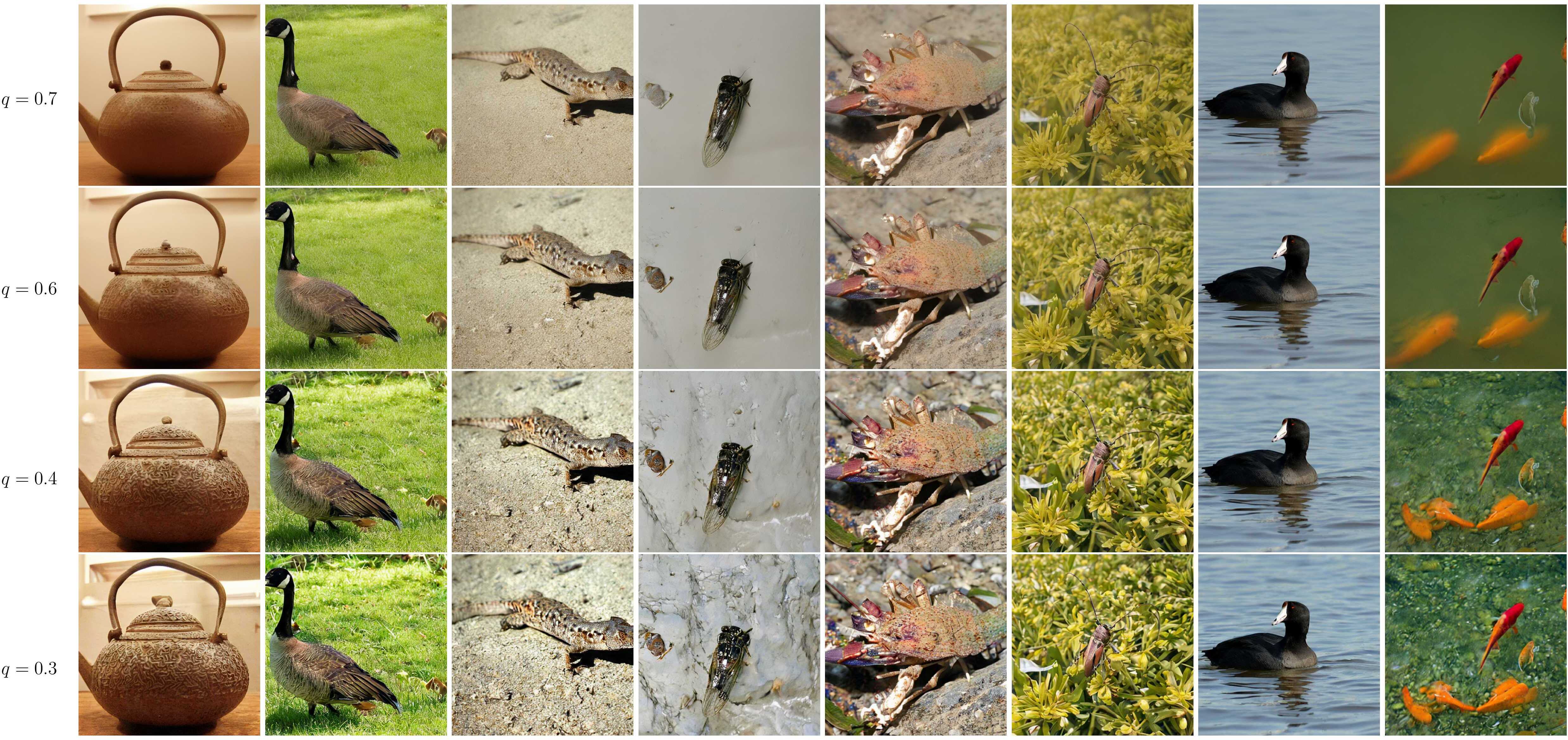
Take-home: Density Guidance modifies the PF-ODE by rescaling the score, achieving fine-grained control of log-density over the entire sampling trajectory.
Stochastic Sampling with Density Guidance
So far, we’ve discussed controlling log-density in deterministic settings. However, stochastic sampling introduces additional challenges and opportunities. In
where
\[\begin{equation}\label{eq:stochastic-guidance-general} \mathbf{u}^{\text{DG-SDE}}_t(\mathbf{x}) = \mathbf{u}^{\text{DG-ODE}}_t(\mathbf{x})+ \underbrace{\frac{1}{2}\varphi^2(t)\frac{\Delta \log p_t(\mathbf{x})}{\| \nabla \log p_t(\mathbf{x}) \|^2}\nabla \log p_t(\mathbf{x})}_{\text{correction for added stochasticity}} \end{equation}\]with \(\mathbf{u}^{\text{DG-ODE}}\) defined in \eqref{eq:dgs} and
\[\begin{equation} P_t(\mathbf{x}) = I - \left(\frac{\nabla \log p_t(\mathbf{x})}{\| \nabla \log p_t(\mathbf{x}) \|}\right) \hspace{-1mm} \left(\frac{\nabla \log p_t(\mathbf{x})}{\| \nabla \log p_t(\mathbf{x}) \|}\right)^T. \end{equation}\]Let’s unpack this. We can add noise to the Density Guidance trajectory, but to maintain the desired evolution of log-density, we have to
- Project the Wiener increment \(d \overline{W}_t\) with \(P_t\) onto the subspace orthogonal to the score;
- Correct the drift for the added stochasticity. To estimate \(\Delta \log p_t(\mathbf{x})=\operatorname{div} \nabla \log p_t(\mathbf{x})\), we use the Hutchinson trick
In practice, we set \(\varphi(t) = \widetilde{\varphi}(t)g(t)\), where \(\widetilde{\varphi}\) specifies the amount of noise relative to \(g\), which is the diffusion coefficient of \eqref{eq:rev-sde}. This simplifies \eqref{eq:stochastic-guidance-general} to
\[\begin{equation} \mathbf{u}^{\text{DG-SDE}}_t(\mathbf{x})=f(t)\mathbf{x} - \frac{1}{2}g^2(t)\left(\eta_t(\mathbf{x})-\widetilde{\varphi}^2(t)\frac{\Delta \log p_t(\mathbf{x})}{\| \nabla \log p_t(\mathbf{x}) \|^2}\right)\nabla \log p_t(\mathbf{x}), \end{equation}\]which again boils down to the PF-ODE \eqref{eq:pf-ode} with an appropriately rescaled score function.
This is particularly useful for balancing detail and variability in generated samples. For example:
- Adding noise early (\(\widetilde{\varphi}(t) \neq 0\) for large \(t\)) in the sampling process introduces variation in high-level features like shapes.
- Adding noise later (\(\widetilde{\varphi}(t) \neq 0\) for small \(t\)) affects only low-level details like texture.
Our method ensures that the log-density evolution remains consistent with the deterministic Density Guidance, allowing precise control while injecting controlled randomness.
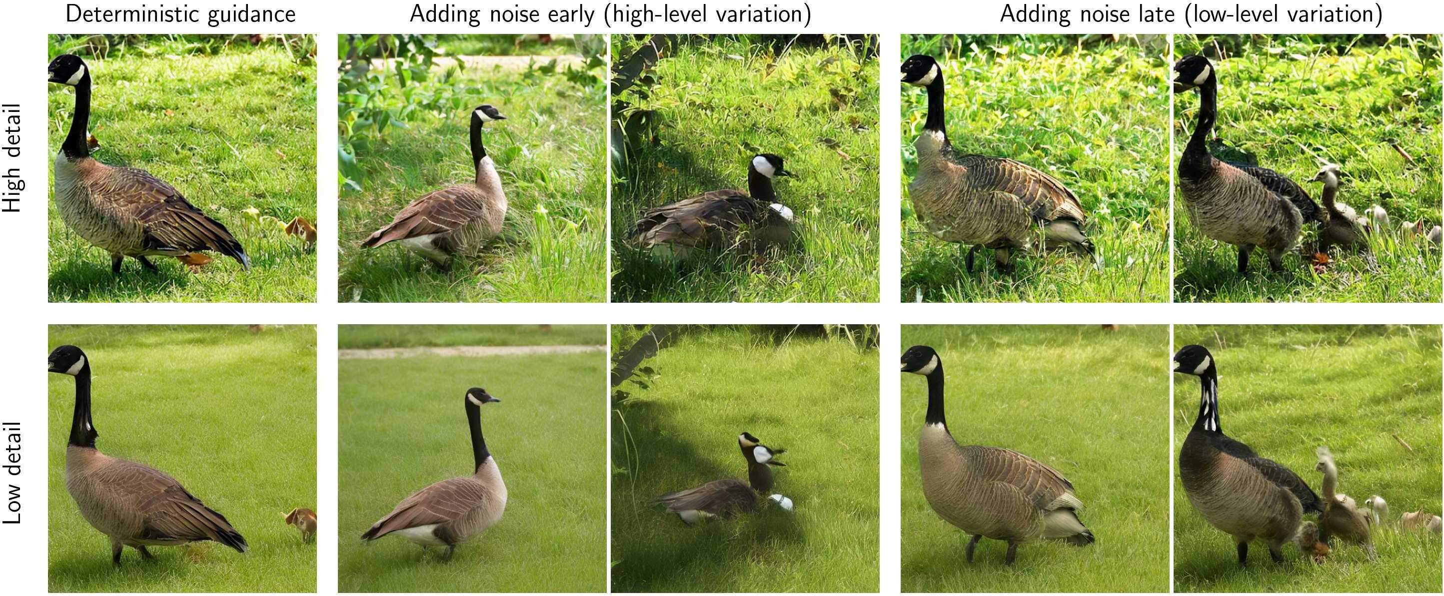
Take-home: Stochastic Density Guidance = same rescaled score approach, plus a projected noise term that preserves the intended log-density schedule.
An interesting observation
Score Alignment
Score alignment measures the angle between:
- \(\nabla \log p_T(\mathbf{x}_T)\) (score of noise distribution) pushed forward via the flow of PF-ODE \eqref{eq:pf-ode} to \(t = 0\), and
- \(\nabla \log p_0(\mathbf{x}_0)\) (score of data distribution).
Let’s clarify what we mean by the “push forward”. Suppose we have a curve \(\gamma\) passing through \(\mathbf{x}_T\), with velocity \(\nabla \log p_T(\mathbf{x}_T)\), i.e. \(\gamma(0)=\mathbf{x}_T\) and \(\gamma'(0)=\nabla \log p_T(\mathbf{x}_T)\).
The pushforward of \(\nabla \log p_T(\mathbf{x}_T)\) via a map \(F\) is simply the tangent vector of the mapped curve, that is:
\[\frac{d}{ds} F(\gamma(s)) \bigg\rvert_{s=0}.\]In our case, \(F\) is the solution map of the PF-ODE, which maps an initial noise sample \(\mathbf{x}_T\) to a final generated sample \(\mathbf{x}_0\) by solving \eqref{eq:pf-ode}. Thus, the pushforward describes how tangent vectors evolve under the PF-ODE.
If the angle is always acute (less than \(90^{\circ}\)), scaling the latent code at \(t = T\) changes \(\log p_0(\mathbf{x}_0)\) in a monotonic way, explaining the relationship between scaling and image detail.
Take-home: If SA holds, simply rescaling the latent noise \(\mathbf{x}_T\) provides a quick method for increasing or decreasing the final log-density (and thus controlling image detail).
Conclusion
Log-density is a crucial concept in understanding and controlling diffusion models. It measures the level of detail in generated images rather than determining in-distribution likelihood. In
These findings not only advance our theoretical understanding of diffusion models but also open up practical avenues for generating images with fine-grained control over detail and variability.